3.2.2. Distances between Language Locations

This approach to data processing involves the calculation of distances between different locations. Most often it incorporates a multi-dimensional (i.e., dependent on many variables) complex mathematical calculation in order to find the “similarity” measure for a language feature, e.g. dialect, accent etc. A short distance between two locations for a particular language feature indicates more similarity of those locations with respect to that language feature.

Calculating abstract distances between linguistic features is also called Dialectometry. Gusfield (1999) provides algorithms to compare strings, i.e. sequences of symbols, such as the Levenshtein distance (LD), a cutting-edge approach, which is also known as string (edit) distance and is used for instance on the LAMSAS project. Measuring the distance is achieved as the following example shows: if a speaker said [rut] at one location and another speaker said [rʊt] at another location, the LD between the two responses would be "1". If one speaker said [rʊt], and another speaker said [raut], the LD between them would be "2" because there is both a substitution (ʊ -> u) and an insertion (a) in the string. The various possible insertions, deletions, and substitutions can further be weighted to make the LD better reflect the linguistic situation.

A cost, e.g. one, is taken for each operation. Since three operations (substitution, deletion and insertion) are possible, the distance between two strings is the total of all the cost of the operations. The cost is not valued identically in all conditions. For example, the change between a stop and a fricative at the same point of articulation could be weighted low because that will be a substitution of a sound at a different point of articulation. Therefore, the actual distance is a “weighted” sum of operations involved in changing one pronunciation into another.

The calculated distance information can be drawn on the map as weighted lines between locations, e.g., darker lines (low distance) for closely connected locations and lighter lines (high distance) for loosely connected locations. Such a map is presented in figure 5, taken from Kretzschmar (2013) , the dialect variation across large numbers of responses from the entire set of LAMSAS speakers is plotted.

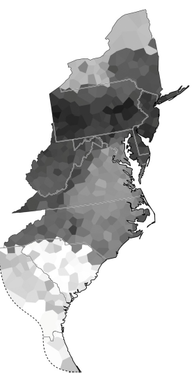
Figure 5: Dialect variation across a large number of responses from the entire set of LAMSAS speakers is calculated using the Levenshtein Distance method

Created with the Personal Edition of HelpNDoc: Full-featured Kindle eBooks generator