Analyzing a data set with three or more interval/ratio scaled variables involves examining all possible combinations of (bivariate) scatterplots. Since the number of plots can be overwhelming, in order to arrange the outcome in a clear way it is convenient to make a single Scatterplot Matrix that depicts all possible scatterplots in one place.
Fig. 18 shows such a matrix for a data set containing five numerical variables. Every single scatterplot is a combination of two of the variables noted in the panels on the main diagonal. For example, panel (2, 1) has the variable ‘Family Size’ on its x-axis and ‘Frequency’ on its y-axis, whereas panel (4, 2) has ‘Length’ on its x-axis and ‘Family Size’ on its y-axis. Another interesting feature of this multipanel view is that since (2, 1) is equivalent to (1, 2) with the axes reversed (compare green boxes in Fig. 17), each pair of variables is plotted twice. Although some statisticians prefer omitting the plots below the diagonal and showing each variable combination only once, there is a good reason for keeping them: as with the interaction plots in section 4.3.2.1., usually one of the two panels is much easier to interpret than the other one, which is why they always should be inspected both (Baayen 2008: 36f.).
The figure was made with pairs(), which requires a data frame with numerical columns as input:
> pairs(data.frame)
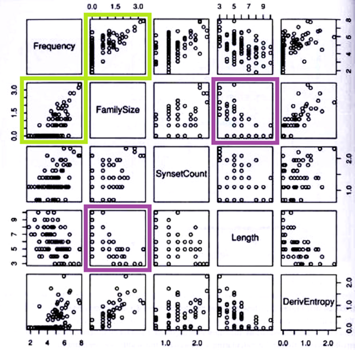
Figure 18: A pairs plot for the five numerical variables in the ratings data frame (modified after Baayen 2008: 36).
Created with the Personal Edition of HelpNDoc: Free EPub and documentation generator