2.1 Methodology

In their chapter, the authors offer four different approaches on how to determine the frequencies of linguistic variants. Given two variants of a variable, form A and form B, their relative frequency can be measured as a fraction of the total (per 1) or as a percentage (per 100). That means that if form A or B has a frequency of 1, the percentage is 100 per cent and the respective other variant does not occur at all. In contrast, a frequency of 0 means the variant does not occur (0 per cent). Of course, more variants are also possible but for convenience only two variants will be used and form B will conventionally be used for the incoming form.

The first method used is pooling. This method implies that the frequency is calculated by dividing the total number of occurrences for one variant by the number of all occurrences of the variable. For example, if the total number of occurrences is 100 and the number of B is 75, the frequency of B would be calculated by dividing 75 by 100 (75/100 = 0.75). Thus, the frequency of form B is 75 per cent or 0.75 whereas form A has a frequency of 25 per cent or 0.25. Of course, linguistic variables are usually more complicated and as the case study will show, the frequencies are usually not as straightforward as portrayed here. Moreover, this method also has some disadvantages which will be discussed later; the main obvious advantage is the easy application of this method.

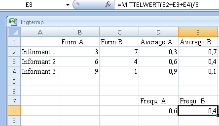
Similar to pooling is the calculation of the average of averages. In this method, the frequency of variants is calculated for each informant (i.e. contributor to the dataset). In the next step, the percentages of all informants are added up and the average of these percentages is calculated by dividing the sum by the number of informants.

When the data is listed in a table, software like Microsoft Excel can easily calculate the average of averages as the following screenshot shows:

The third method of calculating frequency is bootstrapping. It is a method of resampling, which is commonly used in statistics. It means that already calculated values are randomly mixed, i.e. resampled in order to show a frequency estimate. This differs from the two methods mentioned before as the results are different ranges of frequencies, while pooling and the average of averages only provide central tendencies as points without indications of variance.

The last method introduced by the authors is the Bayesian approach. In this approach it is assumed that each frequency has the same probability as other ones. Furthermore it distinguishes between a population frequency and an individual frequency of the variant. In the next step these two frequencies are combined and thus create an interval of the form that is examined (Mannila, Nevalainen and Raumolin-Brunberg 2013:  342-343). This method, just like bootstrapping, produces confidence intervals for the frequencies and thus is different from pooling and average of averages, which only provide a point estimate rather than intervals that show the different ranges of frequencies for the variants. As the Bayesian and bootstrap approaches create similar results and only small deviations, Mannila, Nevalainen and Raumolin-Brunberg suggest only using the easier method of bootstrapping (2013: 21). In this paper, the Bayesian approach will not be used for this reason.

Created with the Personal Edition of HelpNDoc: What is a Help Authoring tool?